Brief Introduction of Value at Risk (VaR) and Its Implementation in Python

Introduction

In the area of finance, the ability to predict the gain and loss is crucial for making decision in investment. Measuring the Value of Risk (VaR), we can estimate the expectation of profitability with decently high confidence, thus enriching information for further analysis and decision making. However, the definition of the VaR does not specify its computing methodology, but only its properties. Consequently, diverse methods can be applied to compute the VaR, with slightly different results. Currently, the most common methodology is historical method, variance-covariance method, and Monte Carlo simulation method. This article will compute and analysis the VaR with the above three methodologies using the dataset of the stock price of Google in the past years.

---

Data

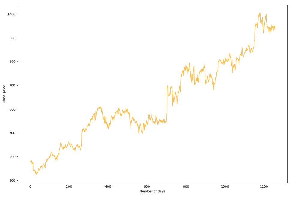
We will use the dataset of everyday stock price from September in 2012 to September in 2017 of the tech company, Google, to illustrate the three different methodologies. The dataset includes the opening, closing, highest and lowest price of that day, and the volume. The data, except the data of volume being integers, are precise to six-digit decimal. The basic trend of data is shown in the picture. To calculate the VaR, we only interested in two area, opening price, and closing price. Both of these determine the return rate, which is essentially what we are interested in.

---

Methodologies

We divided the data into two parts, one for calculating VaR, and another for testing its reliability. The first part of the data consists of 1000 days of data point, and the second part consisted of the rest. Also, in all the following section, we have our confidence level at 95%.

Historical method

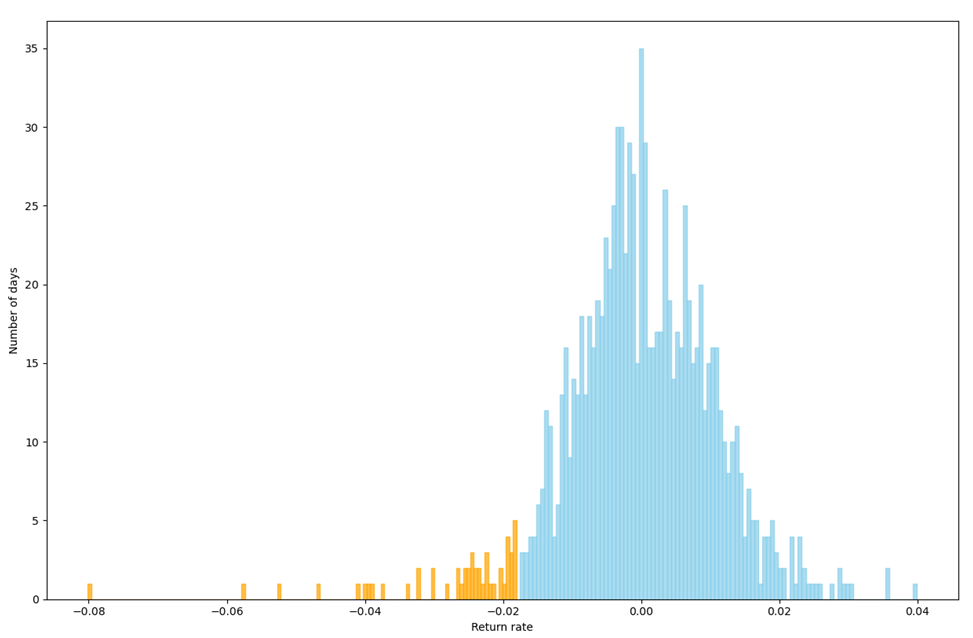
This is a naïve method of prediction with the assumption that the future data will follow the historical trend from a risk perspective. Firstly, it sorts data and marks the 5% percent tail data on the inferior side regarding return rate, because we set the confidence level at 95%. Then, at the separator between the 5% and the rest, it is the VaR calculated from this method, which in this case of Google, describes the 5% low of the return rate of the stock price, indicating that we have 95% confidence that our daily lost will not exceed 1.75%, or when investing $100, we have 95% confidence that our daily lost will not exceed $1.75.

Variance-Covariance Method

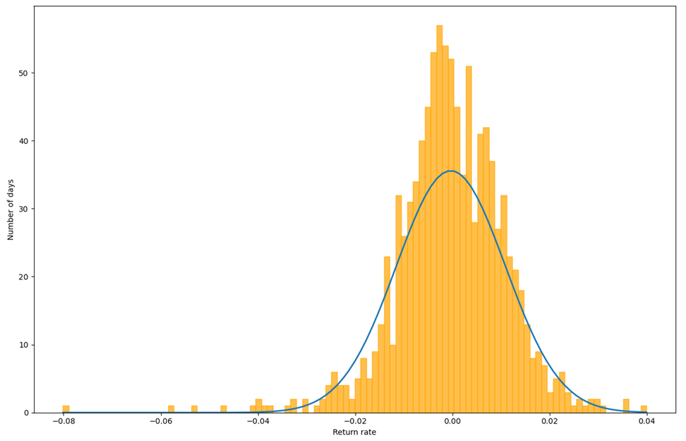
This methodology assumes that the future possibility of the stock is normally distributed. Consequently, to predict the trend of the entity price, we need to know the two element that determine the normal distribution which is the expected return and standard deviation. Eventually, we use the metadata to compute the above two elements and with the resulting normal distribution graph, we separate the data based on our confidence level, in this case 95%, into 5% worst cases and 95% better cases. The boarder between these two are the VaR that we are looking for.

Monte Carlo simulation Method

Monte Carlo simulation is like randomly throw darts at target board and count the scores, giving non-deterministic results. In practice, we randomly choose samples across the dataset. In our example of Google, we randomly choose date points for 100 times and find their 5% worst, determining their VaR. However, Monte Carlo simulation does not specify many aspects of algorithm, and consequently, allows diversified ways of implementation. For example, we may assume the possibility is t-distributed instead of normally distributed, or we may also alter how the exact VaR is computed, like using historical method, rather than Variance-covariance method. But in our implementation, we still assume the future data point if normally distributed and using variance-covariance method for VaR calculation.

Monte Carlo simulation can be very helpful when analyzing the dataset with relatively limited number of data point. A single Monte Carlo simulation randomly chooses a predetermined number of samples from the overall dataset and computes their VaR using specified method. To get the final result, Monte Carlo simulation will be conducted many times. Thus, in some certain scenario, despite the limited data point in the dataset, the data points become reusable, manually enriching the data. In our implementation, the program is set to give one simulation result after averaging 1000 simulation run with 100 samples each.

We also want to find out the consistency by testing the relation between sample size, number of simulation and average VaR and their standard deviation. To examine this, we set the parameter and run the test for 100 times, noting the result. For example, in one of our test runs, we set the sample size to 100 for each nested smaller test and run the nested smaller test 1000 times, averaging all the results, and calculating the deviation. With a repeated 100 times rerunning the Monte Carlo Simulation with above configuration, the average 95% VaR is -1.8525% with a standard deviation of 0.000088.

Because the implementation of Monte Carlo simulation requires lots of repeated sampling and averaging, the performance of such algorithm may be a concern when facing excessive amount of the data points. Consequently, we test the Monte Carlo simulation. The testing for Monte Carlo simulation method measures the running time of the algorithm for 100 runs and calculating the period of one run for every predefined parameter.

---

Data Analysis

Historical method

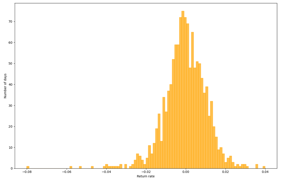
Using Historical method, we get the Figure. The orange bins represent the tail 5% of the data and the light blue bins represent the rest. The separating point lies in -1.7527%, indicating that we have 95% VaR that our daily lose will not exceed the 1.7527%.

Variance-Covariance Method

With Variance-Covariance method, we get the Figure. The orange bins describe the distribution of the return rate, and the blue curve is the normal distribution curve that generated based on the mean and standard deviation from return rate data. From calculation, it shows that with 95% confidence level, we are expecting an at worst 1.8758% of loss, which is a higher expectation of loss than the result from Historical method.

Monte Carlo Simulation Method

The VaR computed with this method is not consist due to the bult-in randomness within code. In a testing run, it gives the result of -1.86% with 95% of confidence. To test its consistency, we run the test with altered parameters and get the following table, noting that number of our testing run for every configuration is always kept 100. Both sample size and number of testing run have three distinguish value, namely, 10, 100, 1000, giving us in total 9 sets of value. After executing the program with predefined parameters, we get the average VaR and the standard deviation for every VaR in the 100-time repeated runs of every configuration.

#	Sample size	# of Test runs	Average VaR	Standard deviation
1	10	10	-0.016808	0.002282
2	10	100	-0.016849	0.000745
3	10	1000	-0.016819	0.000235
4	100	10	-0.018639	0.000819
5	100	100	-0.018502	0.000309
6	100	1000	-0.018540	0.000093
7	1000	10	-0.018778	0.000280
8	1000	100	-0.018725	0.000095
9	1000	1000	-0.018734	0.000029

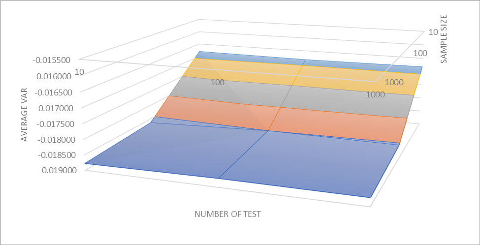
The relation between sample size, number of test run, and average VaR show an interesting trend. Despite the number of testing changes, the corresponding average VaR sees no significant change. However, when sample size is 10, the VaR is drastically different to those of other sample size. Meanwhile, the VaR tends to increase with sample size. Even though with the sample size increases tenfold from 100 to 1000 and the average VaR only increase about 0.0001 in average, the increment is consistent across the test.

# of Simulations Sample size	10	100	1000
10	-0.016808	-0.016849	-0.016819
100	-0.018639	-0.018502	-0.018540
1000	-0.018778	-0.018725	-0.018734

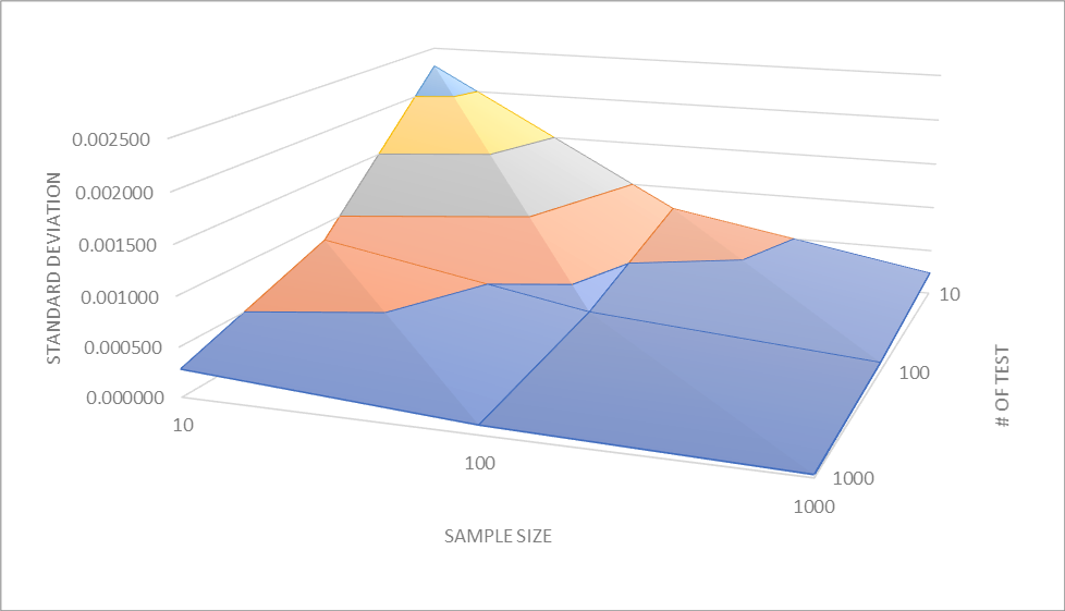
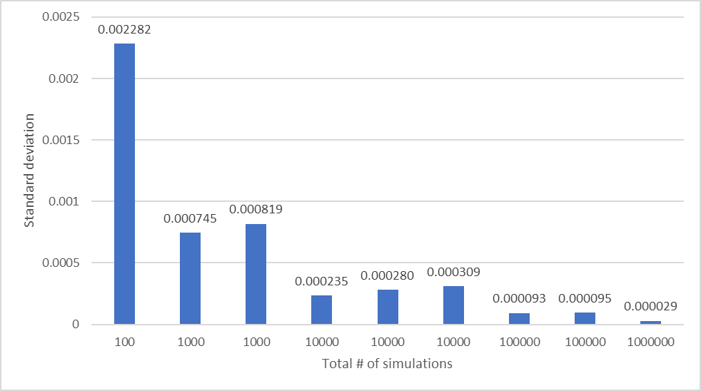
The following table shows the relationship between the number of simulations, sample size, and standard deviation. Intuitively, with the sample size and number of simulations increasing, the deviation among tests is shrinking. The table describing the relationship between the number of simulation and the standard deviation shows the same trend.

# of Simulations Sample size	10	100	1000
10	0.002282	0.000745	0.000235
100	0.000819	0.000309	0.000093
1000	0.000280	0.000095	0.000029

Total # of samples	Standard deviation
100	0.002282
1000	0.000745
1000	0.000819
10000	0.000235
10000	0.000280
10000	0.000309
100000	0.000093
100000	0.000095
1000000	0.000029

Expectation and reality of VaR

VaR does not foresee the future but makes educated guess that decently reflect trend of the data. As shown in the Table 5, the expectation of VaR was in average -1.8268%, but the historical data of the next 200 days reports a VaR of -1.6753%, having some noticeable differences with the expectation. The cause of such difference is obvious, i.e., real-world events may force the stock price of Google does not behave exactly as before. However, despite at most 11% difference, the prediction made by VaR is still accurate to percentile, enabling it to be informative enough for financial decision making.

	Historical method	Variance-covariance method	Monte Carlo simulation method	Standard deviation
First 1000 days	-1.7527%	-1.8758%	-1.8520%	0.000533
Next ~200 days	-1.6753%
Difference	4.4160%	10.6888%	9.5410%

Performance

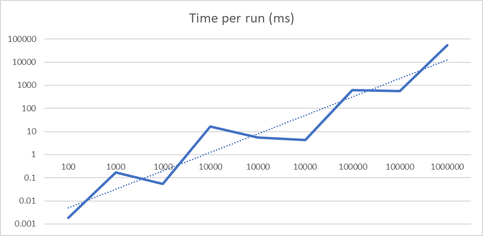
The runtime of Monte Carlo simulation is linear to its total number of samples as expected. However, an interesting trend can be found that with the same amount of the total sample size, more test run shows a worse runtime then more samples per run. However, Table 3 indicates that more simulations also lead to more consistency, indicated by a lower standard deviation. Eventually, the problem becomes which matters more in the real-world application.

# of Simulations Sample size	10	100	1000
10	0.001839	0.16783	16.5796
100	0.05466	5.5147	629.685
1000	4.3104	566.932	53401.59

Total # of samples	Time per run (ms)
100	0.001839
1000	0.167830
1000	0.054660
10000	16.579600
10000	5.514700
10000	4.310400
100000	629.685000
100000	566.932000
1000000	53401.590000

---

Conclusion

The VaR calculated from three methodology shows great similarity across their results, indicating its consistency. Meanwhile, all of three methods of VaR predicts the future VaR reasonably accurate, demonstrating its reliability, except the Monte Carlo simulation method with extremely small sample size. However, despite their resemblance in final results, the Monte Carlo simulation method has an overall worse computing performance because of the large amount of repeated random sampling, while the other two methods process the approximately same level of performance. Moreover, in Monte Carlo simulation method, more samples or more simulation with the same amount of total sample size has a noticeably impact on the consistency and runtime performance of the algorithm. Lastly, the inconsistency of Monte Carlo simulation method requires even more sampling or testing to achieve a reasonable standard deviation across tests, further harming its performance, thus needing performance optimization, like important sampling. Regardless of that, the Monte Carlo simulation provides the most flexibility and can work well with relatively poor data points, allowing for its wide application.

---

Python code

loeeeee/VaR_Monte_Carlo_Simulation: Implementing three methods to calculate VaR (github.com)